Qiskit Primitives

The existing Qiskit interface to backends (backend.run()) was originally designed to accept a list of circuits and return counts for every job. Over time, it became clear that users have diverse purposes for quantum computing, and therefore the ways in which they define the requirements for their computing jobs are expanding.

To address this issue, Qiskit introduced the qiskit.primitives module in version 0.35.0 (Qiskit Terra 0.20.0) to provide a simplified way for end users to compute outputs of interest from a QuantumCircuit and to use backends. Qiskit’s primitives provide methods that make it easier to build modular algorithms and other higher-order programs. Rather than simply returning counts, they return more immediately meaningful information.

The two currently available primitives are the Sampler and the Estimator. The first one simulates a circuit and returns the measurement counts, while the second one calculates and interprets expectation values of quantum operators that are required for many near-term quantum algorithms.

DDSIM provides its own version of these Qiskit primitives that leverage the default circuit simulator based on decision diagrams, while preserving the methods and functionality of the original Qiskit primitives.

Sampler

The Sampler implements the Qiskit BaseSamplerV2 interface. It takes a list of QuantumCircuit objects and simulates them using the CircuitSimulator from MQT DDSIM, returning the measurement counts. The results are encapsulated within a PrimitiveResult object that also contains the job’s metadata.

Furthermore, the Sampler also handles compilation and parameter binding when working with parametrized circuits.

Here, we show an example on how to use this submodule:

import numpy as np
from qiskit import QuantumCircuit
from qiskit.circuit import Parameter

from mqt.ddsim.primitives import Sampler

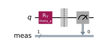
# Parametrized circuit to create an X-gate
theta_a = Parameter("theta_a")
circ = QuantumCircuit(1)
circ.ry(theta_a, 0)
circ.measure_all()

# Show circuit
circ.draw("mpl")

# Initialize sampler
sampler = Sampler()

The run() method accepts an iterable of PUB-like objects, where PUB stands for primitive unified bloc. In the example below, the PUB comprises the circuit and an array of parameter values, where the latter is optional. For more information, see Qiskit’s StatevectorSampler.run(). The number of shots can be set as an additional argument. If not set, the default value is 1024.

pubs = [(circ, [np.pi])]
shots = int(1e4)
job = sampler.run(pubs, shots=shots)
result = job.result()

The result() method of the job returns a PrimitiveResult object. This object contains a SamplerPubResult, which, in turn, contains the measurement counts. It furthermore contains job metadata.

counts = result[0].data["meas"].get_counts()

print(f">>> {result}")
print(f"  > Counts: {counts}")

>>> PrimitiveResult([SamplerPubResult(data=DataBin(meas=BitArray(<shape=(1,), num_shots=10000, num_bits=1>)), metadata={'shots': 10000, 'circuit_metadata': {}})], metadata={'version': 2})
  > Counts: {'1': 10000}

It is also possible to simulate multiple circuits in one job:

# Create a second circuit
circ_2 = QuantumCircuit(1)
circ_2.measure_all()
circ_2.draw("mpl")

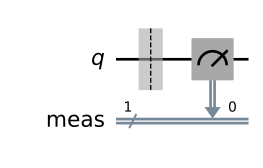
In this case, we have two PUB-like objects.

job = sampler.run([(circ, [np.pi]), circ_2], shots=int(1e4))
result = job.result()

counts_1 = result[0].data["meas"].get_counts()
counts_2 = result[1].data["meas"].get_counts()

print(f">>> {result}")
print(f"  > Counts for circuit 1: {counts_1}")
print(f"  > Counts for circuit 2: {counts_2}")

>>> PrimitiveResult([SamplerPubResult(data=DataBin(meas=BitArray(<shape=(1,), num_shots=10000, num_bits=1>)), metadata={'shots': 10000, 'circuit_metadata': {}}), SamplerPubResult(data=DataBin(meas=BitArray(<shape=(1,), num_shots=10000, num_bits=1>)), metadata={'shots': 10000, 'circuit_metadata': {}})], metadata={'version': 2})
  > Counts for circuit 1: {'1': 10000}
  > Counts for circuit 2: {'0': 10000}

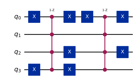
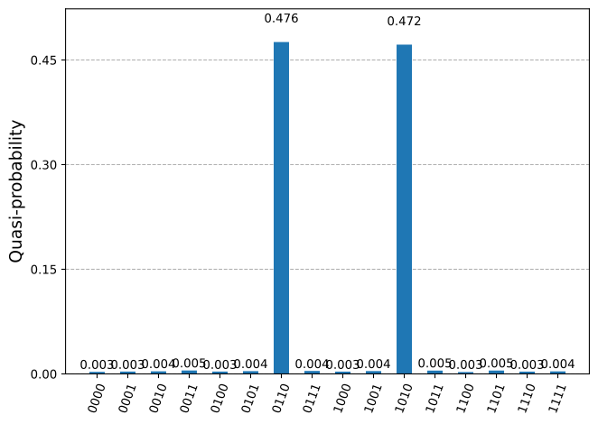
Now, let us use the Sampler on a more complex circuit. For this example, we will test Grover’s algorithm on a 4-qubit circuit where the marked states in the binary representation are “0110” and “1010”.

A similar implementation of Grover’s algorithm using Qiskit’s sampler can be found here: https://learning.quantum.ibm.com/tutorial/grovers-algorithm

# Built-in imports
import math

# Qiskit imports
from qiskit.circuit.library import MCMTGate, GroverOperator, ZGate
from qiskit.visualization import plot_distribution

# Define an oracle circuit that marks the input states, which are represented as a list of bitstrings
def grover_oracle(marked_states: list) -> QuantumCircuit:
    if not isinstance(marked_states, list):
        marked_states = [marked_states]
    # Compute the number of qubits in circuit
    num_qubits = len(marked_states[0])

    qc = QuantumCircuit(num_qubits)
    # Mark each target state in the input list
    for target in marked_states:
        # Flip target bit-string to match Qiskit bit-ordering
        rev_target = target[::-1]
        # Find the indices of all the '0' elements in bit-string
        zero_inds = [ind for ind in range(num_qubits) if rev_target.startswith("0", ind)]
        # Add a multi-controlled Z-gate with pre- and post-applied X-gates (open-controls)
        # where the target bit-string has a '0' entry
        qc.x(zero_inds)
        qc.compose(MCMTGate(ZGate(), num_qubits - 1, 1), inplace=True)
        qc.x(zero_inds)
    return qc

# Enter the states to be marked
marked_states = ["0110", "1010"]
oracle = grover_oracle(marked_states)
oracle.draw("mpl")

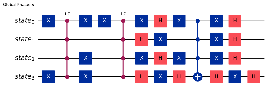
# Build circuit that amplifies the marked states by the oracle
grover_op = GroverOperator(oracle)
grover_op.decompose().draw("mpl")

/tmp/ipykernel_2696/2386812682.py:2: DeprecationWarning: The class ``qiskit.circuit.library.grover_operator.GroverOperator`` is deprecated as of Qiskit 2.1. It will be removed in Qiskit 3.0. Use qiskit.circuit.library.grover_operator instead.
  grover_op = GroverOperator(oracle)

# Compute the optimal number of repetitions of the GroverOperator to amplify the probabilities of the marked states
optimal_num_iterations = math.floor(math.pi / 4 * math.sqrt(2**grover_op.num_qubits / len(marked_states)))

# Build the full Grover circuit
qc = QuantumCircuit(grover_op.num_qubits)
# Create even superposition of all basis states
qc.h(range(grover_op.num_qubits))
# Apply Grover operator the optimal number of times
qc.compose(grover_op.power(optimal_num_iterations), inplace=True)
# Measure all qubits
qc.measure_all()
qc.draw("mpl")

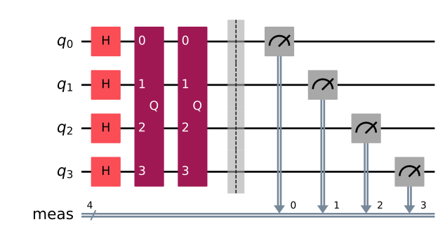
After having built the circuit, use the Sampler to get the measurement counts.

result = sampler.run([qc], shots=int(1e4)).result()
counts = result[0].data["meas"].get_counts()
plot_distribution(counts)

Estimator

The Estimator calculates the expectation value of an observable with respect to a certain quantum state (described by a quantum circuit). It implements the Qiskit BaseEstimatorV2 interface. However, in contrast to Qiskit’s estimator, the DDSIM version exactly computes the expectation value using its simulator based on decision diagrams instead of sampling.

The Estimator also handles parameter binding when dealing with parametrized circuits.

Here, we show an example on how to use it:

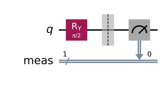
First, we build the observable and the quantum state. The observable is given as a SparsePauliOp object, while the quantum state is described by a QuantumCircuit.

In this example, our observable is the Pauli matrix \(\sigma_{x}\) and the quantum state is \(\frac{1}{\sqrt{2}}(|0\rangle + |1\rangle)\).

import numpy as np
from qiskit import QuantumCircuit
from qiskit.circuit import Parameter
from qiskit.quantum_info import Pauli

from mqt.ddsim.primitives.estimator import Estimator

# Build quantum state
circ = QuantumCircuit(1)
circ.ry(np.pi / 2, 0)
circ.measure_all()

# Build observable
pauli_x = Pauli("X")

# Show circuit
circ.draw("mpl")

# Initialize estimator
estimator = Estimator()

The next step involves running the estimation using the run() method. Just like the run() method of the Sampler, it accepts an iterable of PUB-like objects. In the example below, the QuantumCircuit object representing the quantum state and an array of SparsePauliOp objects representing the observable. If the circuit is parametrized, we would also pass an array of parameters. For more information, see Qiskit’s StatevectorEstimator.run().

# Enter observable and circuit as a sequence
job = estimator.run([(circ, [pauli_x])])
result = job.result()

The result() method of the job returns a PrimitiveResult object. This object contains a PubResult, which, in turn, contains the computed expectation values.

expectation_values = result[0].data["evs"]

print(f">>> {result}")
print(f"  > Expectation values: {expectation_values}")

>>> PrimitiveResult([PubResult(data=DataBin(evs=np.ndarray(<shape=(1,), dtype=float64>), stds=np.ndarray(<shape=(1,), dtype=float64>), shape=(1,)))], metadata={'version': 2})
  > Expectation values: [1.]

Now we explore how the Estimator works with multiple circuits and observables. For this example, we will calculate the expectation value of \(\sigma_{x}\) and \(\sigma_{y}\) with respect to the quantum state \(|1\rangle\). Since our observable list has a length of 2, we need to enter two copies of the QuantumCircuit object representing \(|1\rangle\) as a sequence:

# Build quantum state
circ = QuantumCircuit(1)
circ.ry(np.pi, 0)
circ.measure_all()

# Build observables
pauli_x = Pauli("X")
pauli_y = Pauli("Y")

# Construct pub
pub = (circ, [pauli_x, pauli_y])

# Run estimator
job = estimator.run([pub])
result = job.result()

expectation_values = result[0].data["evs"]

print(f">>> {result}")
print(f"  > Expectation values: {expectation_values}")

>>> PrimitiveResult([PubResult(data=DataBin(evs=np.ndarray(<shape=(2,), dtype=float64>), stds=np.ndarray(<shape=(2,), dtype=float64>), shape=(2,)))], metadata={'version': 2})
  > Expectation values: [0. 0.]

The first and second entries of the list of values are the expectation value of \(\sigma_{x}\) and \(\sigma_{y}\), respectively.

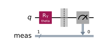
Let us now calculate the expectation values of \(\sigma_{x}\) with respect to \(\frac{1}{\sqrt{2}}(|0\rangle + |1\rangle)\) and \(\frac{1}{\sqrt{2}}(|0\rangle - |1\rangle)\). For this example we will use parametrized circuits to build the quantum state.

theta = Parameter("theta")
circ_2 = QuantumCircuit(1)
circ_2.ry(theta, 0)
circ_2.measure_all()

# Show circuit
circ_2.draw("mpl")

# Construct pub
pub = (circ_2, [pauli_x], [[np.pi / 2], [-np.pi / 2]])

# Run estimator
job = estimator.run([pub])
result = job.result()

expectation_values = result[0].data["evs"]

print(f">>> {result}")
print(f"  > Expectation values: {expectation_values}")

>>> PrimitiveResult([PubResult(data=DataBin(evs=np.ndarray(<shape=(2,), dtype=float64>), stds=np.ndarray(<shape=(2,), dtype=float64>), shape=(2,)))], metadata={'version': 2})
  > Expectation values: [ 1. -1.]