Cat state preparation

Cat states are of quantum states of the form \(|0\rangle^{\otimes w}+|1\rangle^{\otimes w}\) which have various application in quantum error correction, most famously in Shor-style syndrome extraction where a weight-\(w\) stabilizer on a code is measured by performing a transversal CNOT from the support of the stabilizer to a cat state. The difficulty of cat states comes from the fact that it is hard to prepare them in a fault-tolerant manner. If we use cat states for syndrome extraction we want them to be as high-quality as possible.

A cat state can be prepared by preparing one (arbitrary) qubit in the \(|+\rangle\) state and the remaining \(w-1\) in the \(|0\rangle\) state and then entangle the \(|+\rangle\) state with the remaining qubits via CNOT gates. The exact pattern is of these CNOTs is not too important. We just have to make sure that the entanglement spreads to every qubit.

One way to do it is by arranging the CNOTs as a perfect balanced binary tree which prepares the state in \(\log_2{w}\) depth. Let’s define a noisy stim circuit that does this.

import stim
from qiskit import QuantumCircuit

circ = stim.Circuit()
p = 0.05  # physical error rate

def noisy_cnot(circ: stim.Circuit, ctrl: int, trgt: int, p: float) -> None:
    circ.append_operation("CX", [ctrl, trgt])
    circ.append_operation("DEPOLARIZE2", [ctrl, trgt], p)

circ.append_operation("H", [0])
circ.append_operation("DEPOLARIZE1", range(8), p)

noisy_cnot(circ, 0, 4, p)

noisy_cnot(circ, 0, 2, p)
noisy_cnot(circ, 4, 6, p)

noisy_cnot(circ, 0, 1, p)
noisy_cnot(circ, 2, 3, p)
noisy_cnot(circ, 4, 5, p)
noisy_cnot(circ, 6, 7, p)

Show code cell source

Hide code cell source

QuantumCircuit.from_qasm_str(circ.without_noise().to_qasm(open_qasm_version=2)).draw('mpl')

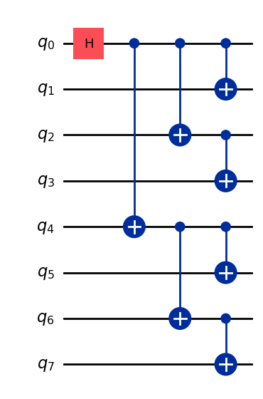
This circuit is not fault-tolerant. A single \(X\)-error in the circuit might spread to high-weight \(X\)-errors. We can show this by simulating the circuit. The cat state is a particularly easy state to analyse because it is resilient to \(Z\)-errors (every \(Z\)-error is equivalent to a weight-zero or weight-one error) and all \(X\) errors simply flip a bit in the state. The distribution of bit flips can be obtained via simulations.

Show code cell source

Hide code cell source

import matplotlib.pyplot as plt
import numpy as np

cat_state = circ.copy()
circ.append_operation("DEPOLARIZE1", range(8), p)
cat_state.append_operation("MR", range(8))

w=8
n_samples = 1000000
sampler = cat_state.compile_sampler()
samples = sampler.sample(n_samples).astype(int)

error_weights = np.min(np.vstack((samples.sum(axis=1), 8 - samples.sum(axis=1))), axis=0)  # at most 4 bits can flip
hist = np.histogram(error_weights, bins=range(4 + 2))[0]/n_samples

x = np.arange(w // 2 + 1)
_fig, ax = plt.subplots()

cmap = plt.cm.plasma
colors = cmap(np.linspace(0, 1, len(x)))

bar_width = 0.8
for xi, yi, color in zip(x, hist, colors):
    ax.bar(
        xi,
        yi,
        width=bar_width,
        color=color,
        alpha=0.8,
        edgecolor="black",
        hatch="//",
        label=f"Error count {xi}" if xi == 0 else "",
    )
    ax.errorbar(xi, yi, fmt="none", capsize=5, color="black", linewidth=1.5)

ax.set_xlabel("Number of errors")
ax.set_ylabel("Probability")
ax.set_xticks(x)
ax.set_yscale("log")
ax.margins(0.2, 0.2)
plt.title(f"Error distribution for w = {w}, p = {p:.2f}")
plt.show()

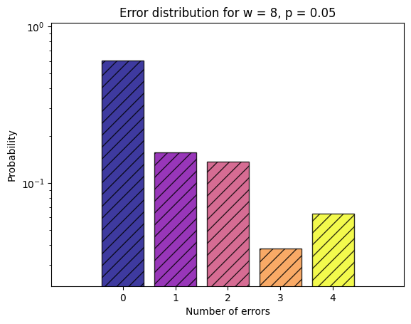
We see that 1,2 and 4 errors occur on the order of the physical error rate, which we set to \(p = 0.05\). Interestingly, 3 errors occur only with a probability of about \(p^2\). This is due to the structure of the circuit. If an \(X\) error occurs, it either propagates to one or two CNOTs, or it doesn’t propagate at all. Three errors are caused by a propagated error and another single-qubit error.

First Attempt at Fault-tolerant Preparation

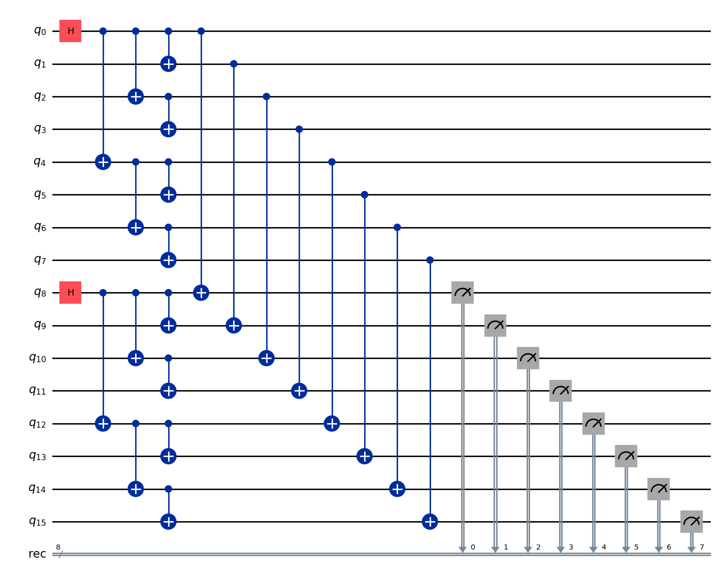
Since the cat-state is CSS, it admits a transversal CNOT. Therefore, we could try to copy the errors of one cat state to another cat state, measure out the qubits of the ancilla state and if we find that an error occurred we restart. QECC provides functionality to set up repeat-until-success cat state preparation experiments.

from mqt.qecc.circuit_synthesis import CatStatePreparationExperiment, cat_state_balanced_tree

w = 8
data = cat_state_balanced_tree(w)
ancilla = cat_state_balanced_tree(w)

experiment = CatStatePreparationExperiment(data, ancilla)

The combined circuit is automatically constructed:

Show code cell source

Hide code cell source

from qiskit.transpiler.passes import RemoveFinalReset
pass_ = RemoveFinalReset()

pass_(pass_(QuantumCircuit.from_qasm_str(experiment.circ.to_qasm(open_qasm_version=2)))).draw('mpl')

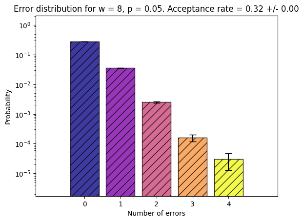
We can now simulate this protocol and look at the error distribution on the data cat state for a specific physical error rate.

experiment.plot_one_p(p, n_samples=100000)

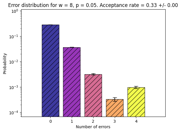
Compared to the above case, the probability of weight-two and weight-four errors has decreased. However, we see that even though about 60% of states are discarded, the weight-four error on the data still occurs about as often on the data as a weight-two error. The reason for this is that both the data and the ancilla state are prepared using the same circuit structure. Consequently, they will have the same set of faults resulting from errors propagating through the circuit. Identical weight-four errors can then cancel out on the ancilla via the transversal CNOT and are subsequently not detected by the ancilla measurement. The situation is illustrated in this crumble circuit.

Second Attempt at Fault-Tolerant State Preparation

The problem in the previous construction is that both circuits propagate errors in the same way. We can try to fix this in one of two ways:

• Prepare the ancilla with a different circuit.

• Permute the transversal CNOTs.

The second case is actually a special case of the first one. Permuting how qubits are connected via the transversal CNOT is equivalent to permuting the CNOTs in the ancilla preparation circuit. We want to find a permutation such that no errors cancel each other out anymore.

We have seen that weight-four errors can cancel out in these circuits. There actually only two weight-four errors that can occur as a consequence of a weight-one error in the circuits, namely \(X_0X_1X_2X_3\) and \(X_4X_5X_6X_7\) (these are actually stabilizer equivalent). Therefore, performing the transversal such that it connects qubit \(q_0\) of the data with qubit \(q_7\) of the ancilla and vice versa should avoid that the weight-four errors cancel out.

In QECC we can pass a permutation on integers \(0, \cdot, w-1\) to the CatStatePreparationExperiment object during construction.

perm = [7,1,2,3,4,5,6,0]

experiment = CatStatePreparationExperiment(data, ancilla, perm)

Again, we can look at the circuit that was actually constructed.

Show code cell source

Hide code cell source

pass_(pass_(QuantumCircuit.from_qasm_str(experiment.circ.to_qasm(open_qasm_version=2)))).draw('mpl')

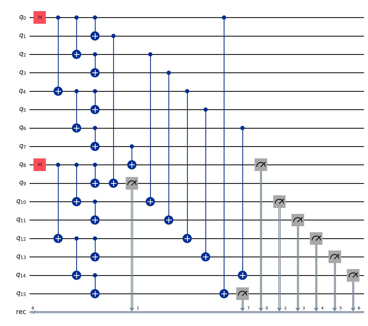
Simulating the circuits shows that now residual weight-four errors on the data are highly unlikely.

experiment.plot_one_p(p, n_samples=100000)

It worked! And it doesn’t even come at the cost of a lower acceptance rate.

Preparing larger cat states

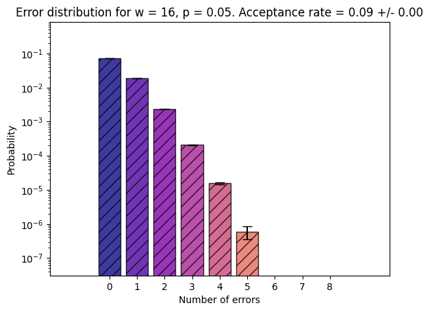
The question now is whether we can make this work for higher-weight cat states. With the framework in place, we can just plug in higher-weight cat states and try different permutations. Let’s consider the case of \(w=16\) and try the following:

• \(\pi_1 = \mathrm{id}\)

• \(\pi_2 = (0 \quad 15)\)

• \(\pi_2 = \begin{pmatrix} 0 & 1 & 2 & 3 & 4 & 5 & 6 & 7 & 8 & 9 & 10 & 11 & 12 & 13 & 14 & 15\\ 0 & 1 & 6 & 10 & 12 & 3 & 5 & 15 & 2 & 8 & 11 & 14 & 4 & 9 & 12 & 7 \end{pmatrix}\)

from mqt.qecc.circuit_synthesis import CatStatePreparationExperiment, cat_state_balanced_tree

w = 16
data = cat_state_balanced_tree(w)
ancilla = cat_state_balanced_tree(w)

pi_1 = list(range(w))

pi_2 = list(range(w))
pi_2[0] = 15
pi_2[15] = 0

pi_3 = [0, 1, 6, 10, 13, 3, 5, 15, 2, 8, 11, 14, 4, 9, 12, 7]

e_1 = CatStatePreparationExperiment(data, ancilla, pi_1)
e_2 = CatStatePreparationExperiment(data, ancilla, pi_2)
e_3 = CatStatePreparationExperiment(data, ancilla, pi_3)

Let’s see the distribution for the identity permutation \(\pi_1\) first.

Show code cell source

Hide code cell source

e_1.plot_one_p(p, n_samples=10000000)

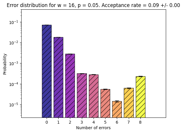
At \(p=0.05\) we only accept about \(12\%\) of all states. We also see that while errors of weight three or higher are less likely as lower-weight errors, the distribution shows that higher-weight errors all occur more or less similarly often.

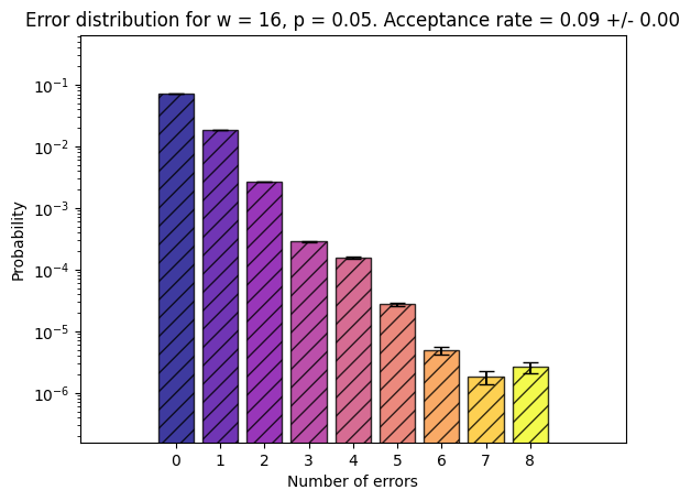
When we permute the transversal CNOT slightly according to \(\pi_2\), we also suppress the errors to some extent.

Show code cell source

Hide code cell source

e_2.plot_one_p(p, n_samples=10000000)
print(e_2.circ.to_crumble_url())

https://algassert.com/crumble#circuit=H_0;CX_0_8_0_4_0_2_0_1_2_3_4_6_4_5_6_7_8_12_8_10_8_9_10_11_12_14_12_13_14_15;H_16;CX_16_24_16_20_16_18_16_17_18_19_20_22_20_21_22_23_24_28_24_26_24_25_26_27_28_30_28_29_30_31_0_31_1_17_2_18_3_19_4_20_5_21_6_22_7_23_8_24_9_25_10_26_11_27_12_28_13_29_14_30_15_16;MR_16_17_18_19_20_21_22_23_24_25_26_27_28_29_30_31_

We see that simply exchanging two qubits is not sufficient to protect the \(w=16\) cat state against higher-weight errors cancelling out. There are, in fact many undetected weight-four errors that lead to a residual error of higher weight on the data qubits. One example is shown in this crumble circuit.

Since there are fewer combinations of errors that cancel out in such a fashion, the error rate still declines, but for a fault-tolerant preparation we would wish for an error of weight \(t\) on the data to occur with probability \(O(p^t)\)

Applying \(\pi_3\) actually yields the desired result:

Show code cell source

Hide code cell source

e_3.plot_one_p(p, n_samples=10000000)

At some point, high-weight errors are so unlikely that they do not occur during the simulation. Getting a better error estimate therefore requires a larger sample-size. Furthermore, to get an estimate of the scaling of the probability of a residual error of a certain size on the data requires sampling at different physical error rates. The cat_prep_experiment method of the CatStatePreparationExperiment class returns the histogram over multiple physical error rates.

Permuting the connectivity of the transversal CNOT is not the only way to improve the robustness of non-deterministic cat state preparation. Another way would be to use different circuits or combine the two methods. The CatStatePreparationExperiment class is intended for evaluating such different preparation schemes.