Cat state preparation

Cat states are of quantum states of the form \(|0\rangle^{\otimes w}+|1\rangle^{\otimes w}\) which have various application in quantum error correction, most famously in Shor-style syndrome extraction where a weight-\(w\) stabilizer on a code is measured by performing a transversal CNOT from the support of the stabilizer to a cat state. The difficulty of cat states comes from the fact that it is hard to prepare them in a fault-tolerant manner. If we use cat states for syndrome extraction we want them to be as high-quality as possible.

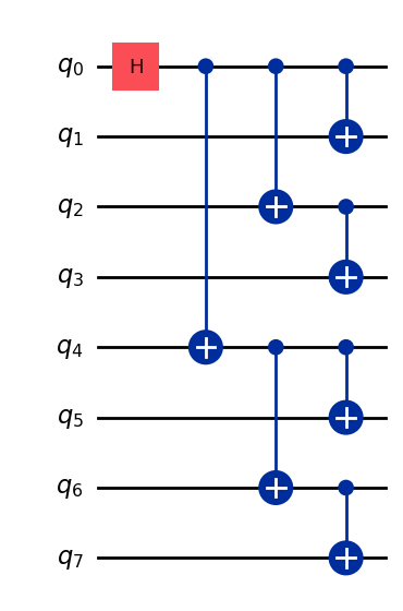
A cat state can be prepared by preparing one (arbitrary) qubit in the \(|+\rangle\) state and the remaining \(w-1\) in the \(|0\rangle\) state and then entangle the \(|+\rangle\) state with the remaining qubits via CNOT gates. The exact pattern is of these CNOTs is not too important. We just have to make sure that the entanglement spreads to every qubit.

One way to do it is by arranging the CNOTs as a perfect balanced binary tree which prepares the state in \(\log_2{w}\) depth. Let’s define a noisy stim circuit that does this.

import stim
from qiskit import QuantumCircuit

circ = stim.Circuit()
p = 0.05  # physical error rate

def noisy_cnot(circ: stim.Circuit, ctrl: int, trgt: int, p: float) -> None:
    circ.append_operation("CX", [ctrl, trgt])
    circ.append_operation("DEPOLARIZE2", [ctrl, trgt], p)

circ.append_operation("H", [0])
circ.append_operation("DEPOLARIZE1", range(8), p)

noisy_cnot(circ, 0, 4, p)

noisy_cnot(circ, 0, 2, p)
noisy_cnot(circ, 4, 6, p)

noisy_cnot(circ, 0, 1, p)
noisy_cnot(circ, 2, 3, p)
noisy_cnot(circ, 4, 5, p)
noisy_cnot(circ, 6, 7, p)

Show code cell source

Hide code cell source

QuantumCircuit.from_qasm_str(circ.without_noise().to_qasm(open_qasm_version=2)).draw('mpl')

This circuit is not fault-tolerant. A single \(X\)-error in the circuit might spread to high-weight \(X\)-errors. We can show this by simulating the circuit. The cat state is a particularly easy state to analyse because it is resilient to \(Z\)-errors (every \(Z\)-error is equivalent to a weight-zero or weight-one error) and all \(X\) errors simply flip a bit in the state.

Show code cell source

Hide code cell source

import matplotlib.pyplot as plt
import numpy as np

cat_state = circ.copy()
circ.append_operation("DEPOLARIZE1", range(8), p)
cat_state.append_operation("MR", range(8))

w=8
n_samples = 1000000
sampler = cat_state.compile_sampler()
samples = sampler.sample(n_samples).astype(int)

error_weights = np.min(np.vstack((samples.sum(axis=1), 8 - samples.sum(axis=1))), axis=0)  # at most 4 bits can flip
hist = np.histogram(error_weights, bins=range(4 + 2))[0]/n_samples

x = np.arange(w // 2 + 1)
_fig, ax = plt.subplots()

cmap = plt.cm.plasma
colors = cmap(np.linspace(0, 1, len(x)))

bar_width = 0.8
for xi, yi, color in zip(x, hist, colors):
    ax.bar(
        xi,
        yi,
        width=bar_width,
        color=color,
        alpha=0.8,
        edgecolor="black",
        hatch="//",
        label=f"Error count {xi}" if xi == 0 else "",
    )
    ax.errorbar(xi, yi, fmt="none", capsize=5, color="black", linewidth=1.5)

ax.set_xlabel("Number of errors")
ax.set_ylabel("Probability")
ax.set_xticks(x)
ax.set_yscale("log")
ax.margins(0.2, 0.2)
plt.title(f"Error distribution for w = {w}, p = {p:.2f}")
plt.show()

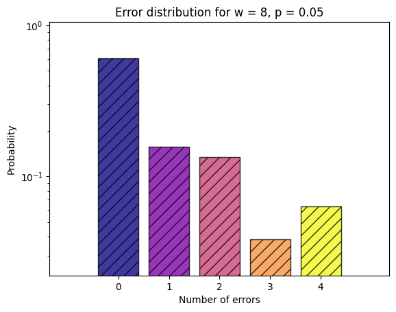
We see that 1,2 and 4 errors occur on the order of the physical error rate, which we set to \(p = 0.05\). In fact, there are about twice as many weight-four errors as there are weight-two errors, since there are four CNOTs that propagate an \(X\) fault to a weight-two error and two CNOTs that propagate an \(X\) fault to a weight-four error. Weight-three errors occur only with a probability of about \(p^2\). This is due to the structure of the circuit. If an \(X\) error occurs, it either propagates to one or two CNOTs, or it doesn’t propagate at all. Three errors are caused by a propagated error and another single-qubit error.

First Attempt at Fault-tolerant Preparation

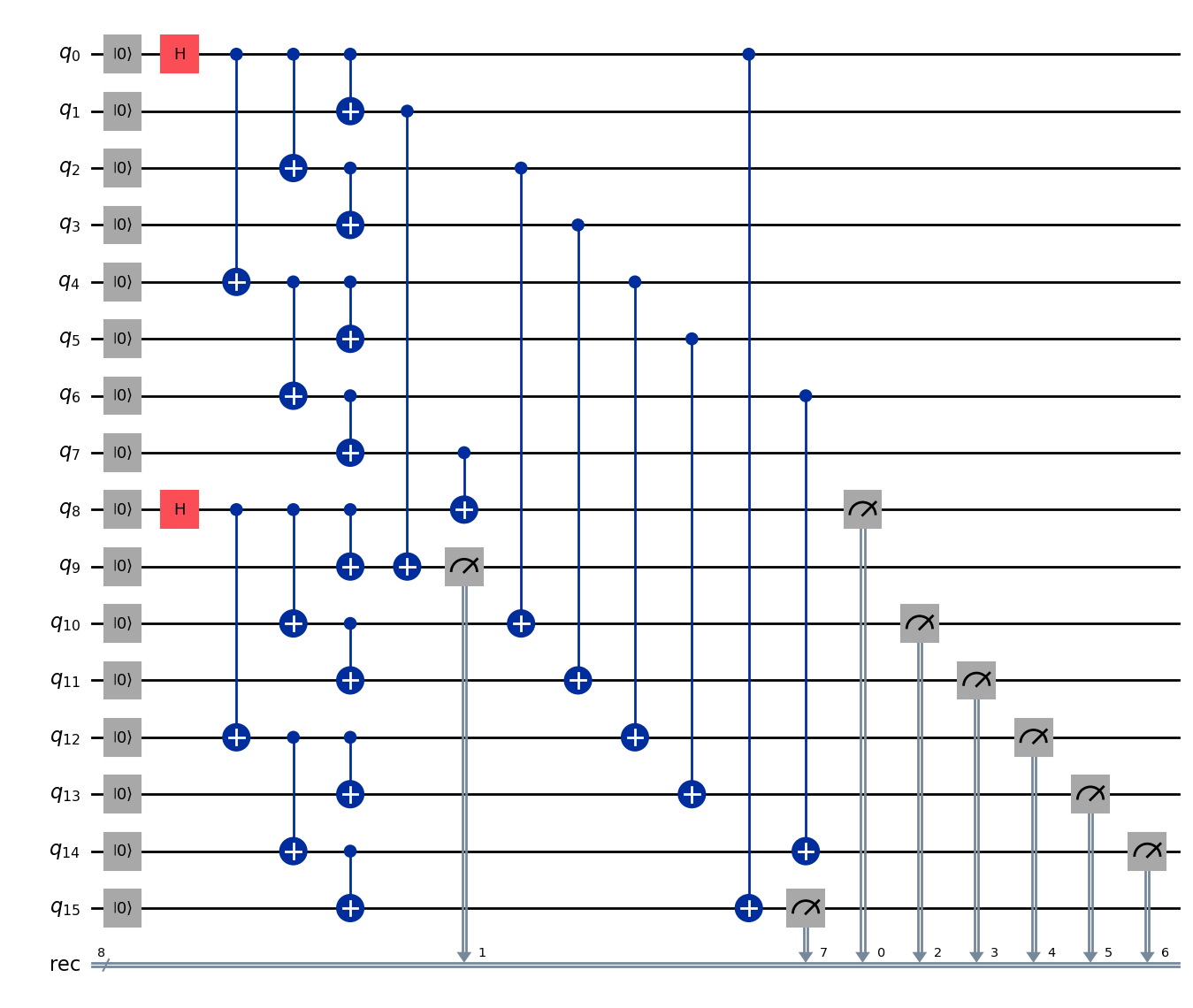
Since the cat-state is CSS, it admits a transversal CNOT. Therefore, we could try to copy the errors of one cat state to another cat state, measure out the qubits of the ancilla state and if we find that an error occurred we restart. QECC provides functionality to set up repeat-until-success cat state preparation experiments.

from mqt.qecc.circuit_synthesis import CatStatePreparationExperiment, cat_state_balanced_tree

w = 8
data = cat_state_balanced_tree(w)
ancilla = cat_state_balanced_tree(w)

experiment = CatStatePreparationExperiment(data, ancilla)

The combined circuit is automatically constructed:

Show code cell source

Hide code cell source

from qiskit.transpiler.passes import RemoveFinalReset
pass_ = RemoveFinalReset()

pass_(pass_(QuantumCircuit.from_qasm_str(experiment.circ.to_qasm(open_qasm_version=2)))).draw('mpl')

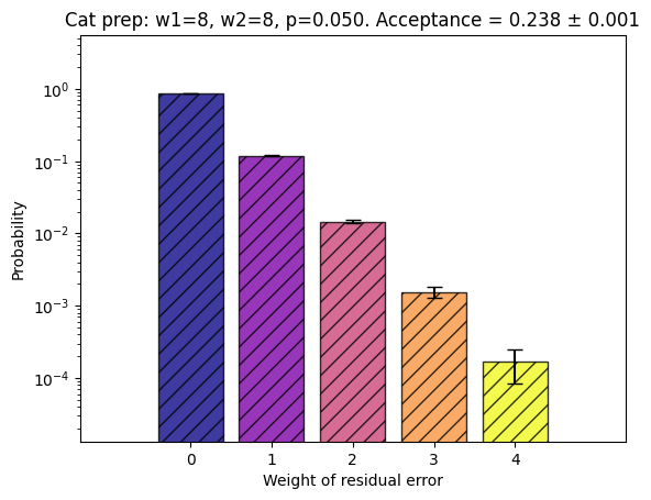
We can now simulate this protocol and look at the error distribution on the data cat state for a specific physical error rate.

experiment.plot_one_p(p, n_samples=100000)

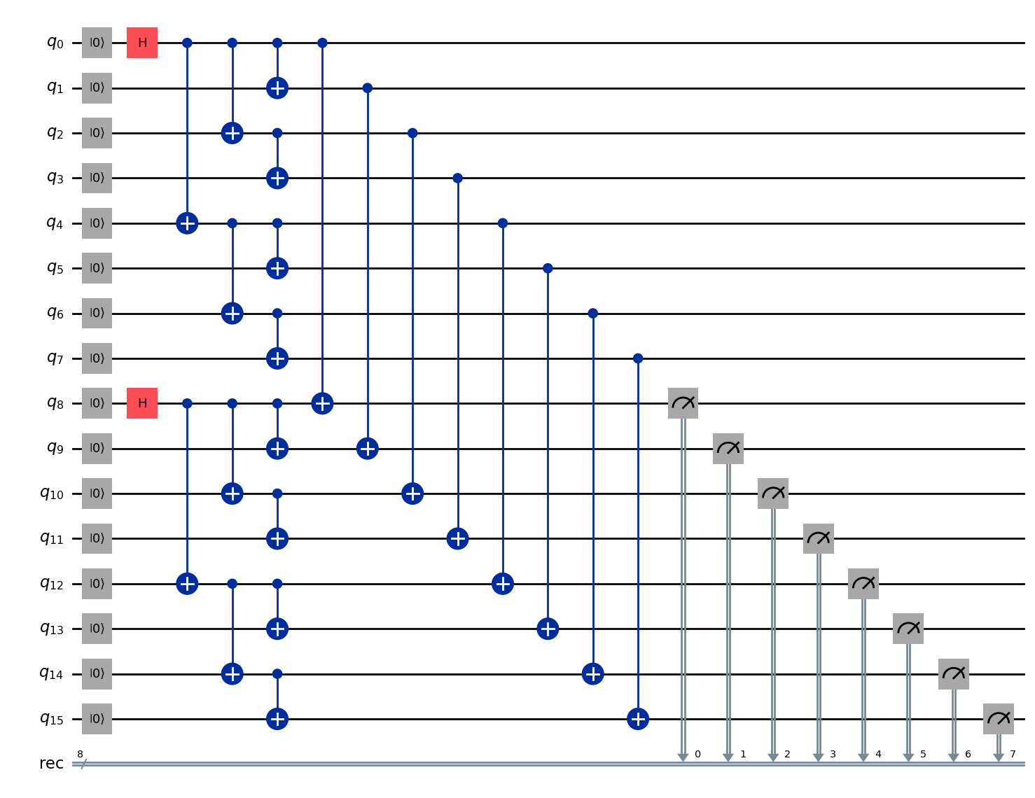
Compared to the above case, the probability of weight-two and weight-four errors has decreased. However, we see that even though about 60% of states are discarded, the weight-four error on the data still occurs about as often on the data as a weight-two error. The reason for this is that both the data and the ancilla state are prepared using the same circuit structure. Consequently, they will have the same set of faults resulting from errors propagating through the circuit. Identical weight-four errors can then cancel out on the ancilla via the transversal CNOT and are subsequently not detected by the ancilla measurement. The situation is illustrated in this crumble circuit.

Second Attempt at Fault-Tolerant State Preparation

The problem in the previous construction is that both circuits propagate errors in the same way. We can try to fix this in one of two ways:

• Prepare the ancilla with a different circuit.

• Permute the transversal CNOTs.

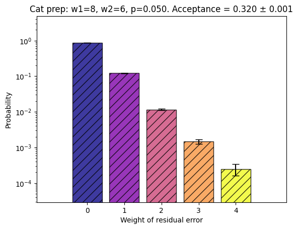
Permuting how qubits are connected via the transversal CNOT is equivalent to permuting the CNOTs in the ancilla preparation circuit. We want to find a permutation such that no errors cancel each other out anymore.

We have seen that weight-four errors can cancel out in these circuits. There actually only two weight-four errors that can occur as a consequence of a weight-one error in the circuits, namely \(X_0X_1X_2X_3\) and \(X_4X_5X_6X_7\) (these are actually stabilizer equivalent). Therefore, performing the transversal cnot such that it connects qubit \(q_0\) of the data with qubit \(q_7\) of the ancilla and vice versa should avoid that the weight-four errors cancel out.

In QECC we can pass a permutation on integers \(0, \cdot, w-1\) to the CatStatePreparationExperiment object during construction.

perm = [7,1,2,3,4,5,6,0]

experiment = CatStatePreparationExperiment(data, ancilla, perm)

Again, we can look at the circuit that was actually constructed.

Show code cell source

Hide code cell source

pass_(pass_(QuantumCircuit.from_qasm_str(experiment.circ.to_qasm(open_qasm_version=2)))).draw('mpl')

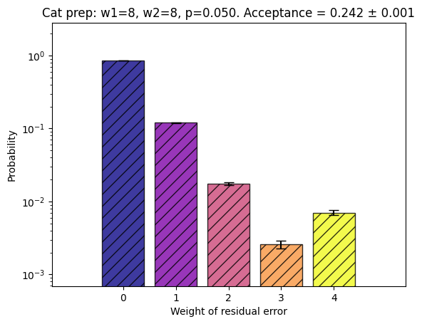
Simulating the circuits shows that now residual weight-four errors on the data are highly unlikely.

experiment.plot_one_p(p, n_samples=100000)

It worked! And it doesn’t even come at the cost of a lower acceptance rate.

Reducing Qubit Overhead

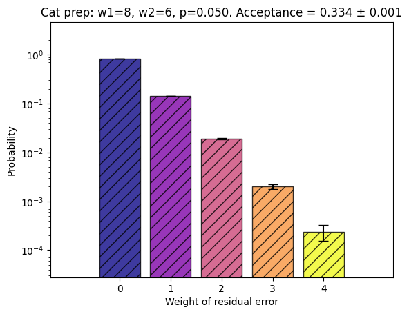
When copying errors from the data to the ancilla cat state, it is not necessary, that the ancilla state has the same size as the data state. In fact, as long as the ancilla state consists of at least two qubits, any transversal CNOT connecting a subset of the data qubits to all ancilla qubits acts trivially on the data state. For the eight qubit case, it turns out that a six qubit ancilla is sufficient. Care still needs to be taken with how the (partial) transversal CNOT is connected.

from mqt.qecc.circuit_synthesis.cat_states import cat_state_pruned_balanced_circuit

w1 = 8
w2 = 6
data = cat_state_pruned_balanced_circuit(w1)
ancilla = cat_state_pruned_balanced_circuit(w2)

ctrls = [1,2,3,5,6,7]
perm = [2,5,0,4,3,1]
experiment = CatStatePreparationExperiment(data, ancilla, perm, ctrls)
experiment.plot_one_p(p, n_samples=100000)

Preparing larger cat states

Constructing fault tolerant partial transversal CNOTs and finding the required ancilla sizes for given cat state preparation circuits becomes more difficult at higher qubit counts and fault distances. QECC has functions for finding such CNOTs automatically.

The most general search approach is search_ft_cnot_cegar which uses counterexample-guided abstraction refinement (CEGAR) to construct both a selection of control qubits and the fault-tolerant permutation at the same time.

from mqt.qecc.circuit_synthesis.cat_states import search_ft_cnot_cegar

t = 4
ctrls, perm, _ = search_ft_cnot_cegar(data, ancilla, t)

experiment = CatStatePreparationExperiment(data, ancilla, perm, ctrls)
experiment.plot_one_p(p, n_samples=100000)

The search_ft_cnot_local_search method uses a heuristic local repair strategy to find fault-tolerant CNOTs. This is faster than the CEGAR approach but is not guaranteed to converge:

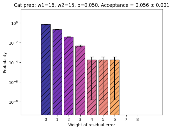
from mqt.qecc.circuit_synthesis.cat_states import search_ft_cnot_local_search

w1 = 16
w2 = 15
t= 8
data = cat_state_pruned_balanced_circuit(w1)
ancilla = cat_state_pruned_balanced_circuit(w2)
ctrls = [0,1,2,3,4,5,6,7,8,9,10,11,12,13,14]
ctrls, perm, _ = search_ft_cnot_local_search(data, ancilla, t, ctrls=ctrls)

experiment = CatStatePreparationExperiment(data, ancilla, perm, ctrls)
experiment.plot_one_p(p, n_samples=100000)

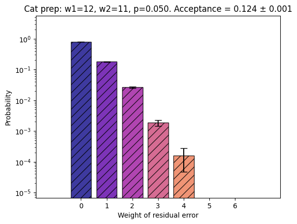
If we already know a good selection of control qubits, performance-wise somewhere in the middle is the search_ft_cnot_smt method, which directly encodes all problematic fault propagations instead of iteratively refining the SMT encoding. Especially for UNSAT instances this usually terminates quickly.

from mqt.qecc.circuit_synthesis.cat_states import search_ft_cnot_smt

w1 = 12
w2 = 11
t= 6
data = cat_state_pruned_balanced_circuit(w1)
ancilla = cat_state_pruned_balanced_circuit(w2)
ctrls, perm, _ = search_ft_cnot_smt(data, ancilla, t)

experiment = CatStatePreparationExperiment(data, ancilla, perm, ctrls)
experiment.plot_one_p(p, n_samples=100000)

Loading already Constructed FT Cat States

To avoid redoing redundant computations, stim circuits for cat states of sizes up \(49\) qubits and fault distances up to \(9\) can be found here. There is also a json file which explicitly lists control qubits and target permutation for a given combination of data cat state size (\(w_1\)), ancilla cat state size (\(w_2\)) and fault distance (\(t\)).