Memory Surrogate Training and Prediction

For control sequences beyond what you can simulate exhaustively, train a causal Transformer surrogate on Hamiltonian rollouts of the open system. predict() returns the reduced density matrix of the probe qubit after a control sequence.

Surrogate training requires PyTorch (pip install mqt.yaqs[torch]). Over short temporal horizons (few intervention steps), compare surrogate rollouts to Hamiltonian training targets and to exact dense or MPO process tensors built with build_process_tensor(). Environmental memory probing (characterize) is covered in Probing Environmental Memory.

Warning

Exact references scale exponentially with sequence length. Use them only over few intervention steps — short probes in time, not long open-system runs.

Setup

import matplotlib.pyplot as plt
import numpy as np

from mqt.yaqs import AnalogSimParams, Hamiltonian, MemoryCharacterizer
from mqt.yaqs.characterization.memory.backends.surrogates.workflow import build_training_dataset
from mqt.yaqs.characterization.memory.shared.encoding import encode_rho_pauli, unpack_rho8
from mqt.yaqs.characterization.memory.shared.metrics import mean_trace_distance_rho8
from mqt.yaqs.core.data_structures.mpo import MPO

PAULI_Z = np.array([[1, 0], [0, -1]], dtype=np.complex128)


def z_expectation(rho8_row: np.ndarray) -> float:
    """Return ⟨Z⟩ from a packed 8-float density-matrix row."""
    rho = unpack_rho8(rho8_row)
    return float(np.trace(PAULI_Z @ rho).real)

length = 2
ham = Hamiltonian.ising(length=length, J=1.0, g=1.0)
params = AnalogSimParams(dt=0.1)
mc = MemoryCharacterizer(show_progress=False)
num_interventions = 2
timesteps = [0.0, 0.0, 0.0]
intervention_style = "measure_prepare"

Use a probe + environment chain (length >= 2). Match intervention_style and timesteps between training, predict, and build_process_tensor (length num_interventions + 1).

Train a surrogate

Training fixes num_interventions on the model — the horizon the network was fit to. The settings below mirror the accuracy regression in the test suite (measure_prepare legs, short schedule).

model = mc.train(
    ham,
    params,
    num_interventions=num_interventions,
    n=60,
    seed=0,
    timesteps=timesteps,
    intervention_style=intervention_style,
    train_kwargs={
        "epochs": 120,
        "batch_size": 16,
        "lr": 2e-3,
        "device": "cpu",
        "prefix_loss": "full",
    },
    model_kwargs={
        "d_model": 32,
        "nhead": 4,
        "num_layers": 1,
        "dim_ff": 64,
        "dropout": 0.0,
    },
)

Evaluate on held-out Hamiltonian rollouts

Generate fresh training sequences with a different seed and compare the surrogate’s final-step predictions to the Hamiltonian targets used during dataset construction:

held_out = build_training_dataset(
    MPO.ising(length=length, J=1.0, g=1.0),
    params,
    num_interventions=num_interventions,
    n=60,
    seed=999,
    intervention_style=intervention_style,
    show_progress=False,
    timesteps=timesteps,
)
e_test, rho0_test, rho_true = held_out.tensors
rho_pred = model.predict(e_test.numpy(), rho0_test.numpy(), return_numpy=True)

z_true = np.array([z_expectation(row) for row in rho_true.numpy()[:, -1, :]])
z_pred = np.array([z_expectation(row) for row in rho_pred[:, -1, :]])
mean_td = mean_trace_distance_rho8(rho_pred[:, -1, :], rho_true.numpy()[:, -1, :])

fig, ax = plt.subplots(figsize=(4.5, 4))
ax.scatter(z_true, z_pred, s=18, alpha=0.75)
lims = (min(z_true.min(), z_pred.min()) - 0.05, max(z_true.max(), z_pred.max()) + 0.05)
ax.plot(lims, lims, "k--", linewidth=1)
ax.set_xlim(lims)
ax.set_ylim(lims)
ax.set_xlabel(r"Hamiltonian $\langle Z \rangle$ (final step)")
ax.set_ylabel(r"Surrogate $\langle Z \rangle$ (final step)")
ax.set_title(rf"Held-out rollouts (mean trace distance = {mean_td:.3f})")
ax.set_aspect("equal")
fig.tight_layout()

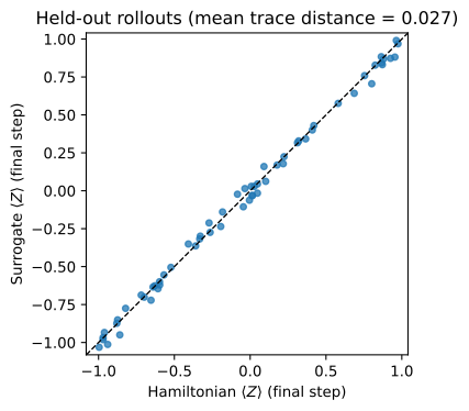
Compare explicit control sequences

The usual workflow after training is to call predict() with your own control sequence and compare outcomes across choices. Train a one-leg surrogate on random unitary controls, then pass different explicit unitary lists to the same model. This mirrors the quickstart workflow (Quickstart) with the longer training budget used above:

unitary_timesteps = [0.0, 0.0]
controls_model = mc.train(
    ham,
    params,
    num_interventions=1,
    n=120,
    seed=2,
    timesteps=unitary_timesteps,
    intervention_style="haar",
    train_kwargs={
        "epochs": 120,
        "batch_size": 16,
        "lr": 2e-3,
        "device": "cpu",
        "prefix_loss": "full",
    },
    model_kwargs={
        "d_model": 32,
        "nhead": 4,
        "num_layers": 1,
        "dim_ff": 64,
        "dropout": 0.0,
    },
)

rho0_controls = np.eye(2, dtype=np.complex128) / 2.0
hadamard = np.array([[1, 1], [1, -1]], dtype=np.complex128) / np.sqrt(2)
pauli_x = np.array([[0, 1], [1, 0]], dtype=np.complex128)
control_sequences = {
    r"$\mathrm{H}$": [{"unitary": hadamard}],
    r"$\mathrm{X}$": [{"unitary": pauli_x}],
}

pauli_ops = {
    "X": np.array([[0, 1], [1, 0]], dtype=np.complex128),
    "Y": np.array([[0, -1j], [1j, 0]], dtype=np.complex128),
    "Z": np.array([[1, 0], [0, -1]], dtype=np.complex128),
}
expectations = {
    label: [
        float(np.trace(op @ mc.predict(controls_model, rho0_controls, controls, num_interventions=1)).real)
        for op in pauli_ops.values()
    ]
    for label, controls in control_sequences.items()
}

pauli_names = list(pauli_ops)
x = np.arange(len(pauli_names))
width = 0.35

fig, ax = plt.subplots(figsize=(5.5, 3.5))
for offset, (label, values) in zip((-width / 2, width / 2), expectations.items()):
    ax.bar(x + offset, values, width, label=f"control {label}")
ax.set_xticks(x, pauli_names)
ax.set_ylabel(r"$\langle P \rangle$")
ax.set_title("Probe Pauli expectations for two control sequences")
ax.legend(frameon=False)
fig.tight_layout()

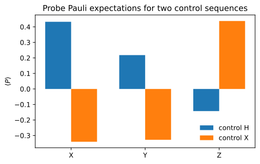
Extend the per-leg list when num_interventions > 1 to probe multi-step sequences (for example [H, X]).

Validate against exact references

Build exhaustive process tensors for the same schedule. For process tensors, rho0 in predict must match pt.initial_rho (the site-0 state after the initial leg of the reference schedule).

Dense and MPO implementations should agree on identical interventions. Compare all three backends on a stochastic sequence drawn from the training style (measure_prepare here): pass a fresh np.random.default_rng(seed) to each predict call (reusing one RNG object advances its state between calls).

pt_dense = mc.build_process_tensor(
    ham, params, timesteps=timesteps, return_type="dense", num_trajectories=48,
)
pt_mpo = mc.build_process_tensor(
    ham, params, timesteps=timesteps, return_type="mpo", num_trajectories=48,
)

rho0 = pt_dense.initial_rho
compare_seed = 7

rho_dense = mc.predict(
    pt_dense, rho0, intervention_style, num_interventions=num_interventions,
    rng=np.random.default_rng(compare_seed),
)
rho_mpo = mc.predict(
    pt_mpo, rho0, intervention_style, num_interventions=num_interventions,
    rng=np.random.default_rng(compare_seed),
)
rho_surrogate = mc.predict(
    model, rho0, intervention_style, num_interventions=num_interventions,
    rng=np.random.default_rng(compare_seed),
)

pauli_labels = [r"$X$", r"$Y$", r"$Z$"]
pauli_dense = encode_rho_pauli(rho_dense)[1:]
pauli_mpo = encode_rho_pauli(rho_mpo)[1:]
pauli_surrogate = encode_rho_pauli(rho_surrogate)[1:]
x = np.arange(len(pauli_labels))
width = 0.25

fig, ax = plt.subplots(figsize=(5.5, 3.5))
ax.bar(x - width, pauli_dense, width, label="dense", color="tab:blue")
ax.bar(x, pauli_mpo, width, label="MPO", color="tab:orange", alpha=0.85)
ax.bar(x + width, pauli_surrogate, width, label="surrogate", color="tab:green", alpha=0.85)
ax.set_xticks(x, pauli_labels)
ax.set_ylabel(r"$\langle P \rangle$")
ax.set_title(
    rf"Matched {intervention_style} sequence ($\|\rho_{{\mathrm{{dense}}}}-\rho_{{\mathrm{{MPO}}}}\|_F$ = "
    rf"{np.linalg.norm(rho_dense - rho_mpo):.1e})"
)
ax.legend(frameon=False)
fig.tight_layout()

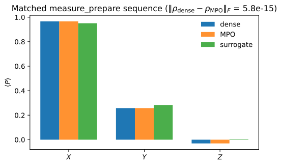
Dense and MPO should overlap; the surrogate approximates the same draw at the reference rho0. Held-out Hamiltonian rollouts above use random probe rho0 values from data generation — a different setup than the fixed reference state baked into process tensors.

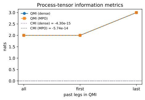
The same information functionals are available on either backend. For this short horizon, conditional mutual information is near zero while QMI grows when more past legs are included:

past_choices = ("all", "first", "last")
qmi_dense = [mc.compute_qmi(pt_dense, past=p) for p in past_choices]
qmi_mpo = [mc.compute_qmi(pt_mpo, past=p) for p in past_choices]
cmi_dense = mc.compute_cmi(pt_dense)
cmi_mpo = mc.compute_cmi(pt_mpo)

fig, ax = plt.subplots(figsize=(5, 3.5))
ax.plot(past_choices, qmi_dense, "o-", label="QMI (dense)")
ax.plot(past_choices, qmi_mpo, "s--", label="QMI (MPO)", alpha=0.85)
ax.axhline(cmi_dense, color="tab:purple", linestyle=":", linewidth=1.5, label=rf"CMI (dense) = {cmi_dense:.2e}")
ax.axhline(cmi_mpo, color="tab:gray", linestyle="--", linewidth=1, label=rf"CMI (MPO) = {cmi_mpo:.2e}")
ax.set_ylabel("nats")
ax.set_xlabel(r"past legs in QMI")
ax.set_title("Process-tensor information metrics")
ax.legend(frameon=False, fontsize=8, loc="upper left")
fig.tight_layout()

Split-cut response matrices and \(S_V(c)\) from Probing Environmental Memory probe the same memory content in an operational setting.

Related topics

• Probing Environmental Memory — split-cut probing, response matrix, reset-delay sweeps

• Quickstart — minimal train/predict snippet

• API reference: :class:~mqt.yaqs.memory_characterizer.MemoryCharacterizer