Trapped-Ion Position-Grid Emulation
This example evolves a single ion on a finite position grid with
trapped_ion(). Each ion is one MPO site;
the local Hilbert space is the grid itself. The Hamiltonian combines a
finite-difference kinetic term and a harmonic trap—see Building Hamiltonians for the
factory API and two-ion Coulomb extensions.
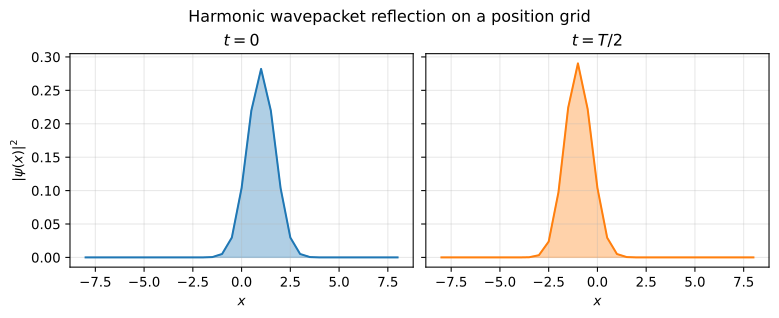
We initialize a displaced harmonic-oscillator wavepacket in a static central well. In the continuum limit, its center follows \(\langle x(t)\rangle = x_0 \cos(\omega t)\), so after half a trap period it reaches the opposite turning point.
1. Hamiltonian and initial state
 1import numpy as np
 2
 3from mqt.yaqs import Hamiltonian, MPO, State
 4
 5omega = 1.0
 6initial_displacement = 1.0
 7half_period = np.pi / omega
 8
 9positions = np.linspace(-8.0, 8.0, 33)
10grid_dim = len(positions)
11
12initial_grid_state = np.exp(-0.5 * (positions - initial_displacement) ** 2).astype(np.complex128)
13initial_grid_state /= np.linalg.norm(initial_grid_state)
14
15hamiltonian = Hamiltonian.from_mpo(MPO.trapped_ion(positions, masses=[1.0], omega=omega))
16state = State(length=1, vector=initial_grid_state, physical_dimensions=[grid_dim])
2. Noiseless evolution to \(T/2\)
 1from mqt.yaqs import AnalogSimParams, Simulator
 2
 3params = AnalogSimParams(
 4    observables=[],
 5    elapsed_time=half_period,
 6    dt=half_period / 16,
 7    max_bond_dim=None,
 8    svd_threshold=1e-12,
 9    krylov_tol=1e-12,
10    preset="exact",
11    get_state=True,
12    sample_timesteps=False,
13)
14
15result = Simulator(show_progress=False).run(state, hamiltonian, params)
16final_state = result.output_state.vector
17final_x = float(np.sum(positions * np.abs(final_state) ** 2))
The final \(\langle x\rangle\) is close to \(-x_0\) but not exact because the simulation uses a finite grid and a finite-difference kinetic operator.
1print(f"Initial <x>       = {initial_displacement:.6f}")
2print(f"Final <x> at T/2  = {final_x:.6f}")
3print(f"Continuum target  = {-initial_displacement:.6f}")
Initial <x>       = 1.000000
Final <x> at T/2  = -0.981441
Continuum target  = -1.000000
3. Wavepacket at \(t=0\) and \(t=T/2\)
 1import matplotlib.pyplot as plt
 2
 3prob_initial = np.abs(initial_grid_state) ** 2
 4prob_final = np.abs(final_state) ** 2
 5
 6fig, axes = plt.subplots(1, 2, figsize=(8, 3.2), layout="constrained", sharey=True)
 7axes[0].fill_between(positions, prob_initial, alpha=0.35, color="tab:blue")
 8axes[0].plot(positions, prob_initial, color="tab:blue", lw=1.5)
 9axes[0].set_title(r"$t = 0$")
10axes[0].set_xlabel(r"$x$")
11axes[0].set_ylabel(r"$|\psi(x)|^2$")
12axes[0].grid(alpha=0.3)
13
14axes[1].fill_between(positions, prob_final, alpha=0.35, color="tab:orange")
15axes[1].plot(positions, prob_final, color="tab:orange", lw=1.5)
16axes[1].set_title(rf"$t = T/2$")
17axes[1].set_xlabel(r"$x$")
18axes[1].grid(alpha=0.3)
19
20fig.suptitle("Harmonic wavepacket reflection on a position grid")
21plt.show()