Weak Circuit Simulation
Weak digital simulation samples computational-basis shots after a noisy circuit evolution, mimicking hardware readout statistics. Use WeakSimParams and read bitstring counts from counts.
For expectation-value simulation and mid-circuit observables, see Strong Simulation. For parameter presets and truncation settings, see Configuring Simulation Parameters.
You can pass an OpenQASM file path or raw OpenQASM string to run() instead of building a qiskit.circuit.QuantumCircuit in Python (OpenQASM 3 requires pip install mqt-yaqs[qasm3]).
1. Circuit
We use a shallow randomized ansatz—single-qubit \(R_y\) rotations followed by a linear chain of \(CZ\) gates—typical of variational benchmarks.
 1import numpy as np
 2from qiskit.circuit import QuantumCircuit
 3
 4num_qubits = 6
 5circuit = QuantumCircuit(num_qubits)
 6rng = np.random.default_rng(42)
 7for i in range(num_qubits):
 8    circuit.ry(float(rng.uniform(0.6, 2.2)), i)
 9for i in range(num_qubits - 1):
10    circuit.cz(i, i + 1)
11circuit.measure_all()
2. Initial state and noise model
1from mqt.yaqs import NoiseModel, State
2
3state = State(num_qubits, initial="zeros")
4
5gamma = 0.5
6noise_model = NoiseModel([
7    {"name": "lowering", "sites": [i], "strength": gamma} for i in range(num_qubits)
8])
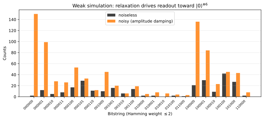
Amplitude damping relaxes each qubit toward \(\ket{0}\). During circuit execution the noise channels compete with unitary spreading, so readout mass shifts toward the all-zeros bitstring compared with the noiseless run.
3. Simulation parameters and run
WeakSimParams requires an explicit shots count (not covered by accuracy presets). We run the same circuit twice: once without noise (ideal readout statistics) and once with on-site amplitude damping.
1from mqt.yaqs import Simulator, WeakSimParams
2
3sim_params = WeakSimParams(shots=1024, max_bond_dim=16, svd_threshold=1e-6, random_seed=7)
4
5sim = Simulator(show_progress=False)
6result_clean = sim.run(state, circuit, sim_params)
7result_noisy = sim.run(state, circuit, sim_params, noise_model)
Measuring shots: 0%| | 0/1024 [00:00<?, ?it/s]
Measuring shots: 5%|█▏ | 53/1024 [00:00<00:01, 529.11it/s]
Measuring shots: 10%|██▎ | 106/1024 [00:00<00:01, 465.97it/s]
Measuring shots: 15%|███▎ | 154/1024 [00:00<00:01, 439.49it/s]
Measuring shots: 20%|████▍ | 208/1024 [00:00<00:01, 474.62it/s]
Measuring shots: 26%|█████▋ | 265/1024 [00:00<00:01, 506.25it/s]
Measuring shots: 31%|██████▊ | 317/1024 [00:00<00:01, 468.83it/s]
Measuring shots: 36%|███████▊ | 365/1024 [00:00<00:01, 463.85it/s]
Measuring shots: 41%|█████████ | 422/1024 [00:00<00:01, 493.10it/s]
Measuring shots: 46%|██████████▏ | 475/1024 [00:00<00:01, 500.67it/s]
Measuring shots: 51%|███████████▎ | 526/1024 [00:01<00:01, 469.41it/s]
Measuring shots: 56%|████████████▎ | 574/1024 [00:01<00:01, 448.18it/s]
Measuring shots: 61%|█████████████▍ | 628/1024 [00:01<00:00, 473.36it/s]
Measuring shots: 67%|██████████████▋ | 686/1024 [00:01<00:00, 501.42it/s]
Measuring shots: 72%|███████████████▉ | 742/1024 [00:01<00:00, 517.78it/s]
Measuring shots: 78%|█████████████████▏ | 798/1024 [00:01<00:00, 528.77it/s]
Measuring shots: 83%|██████████████████▎ | 852/1024 [00:01<00:00, 487.29it/s]
Measuring shots: 88%|███████████████████▍ | 902/1024 [00:01<00:00, 463.73it/s]
Measuring shots: 93%|████████████████████▍ | 950/1024 [00:01<00:00, 447.34it/s]
Measuring shots: 98%|████████████████████▌| 1004/1024 [00:02<00:00, 469.73it/s]
Measuring shots: 100%|█████████████████████| 1024/1024 [00:02<00:00, 479.83it/s]
For log-normal disorder on relaxation rates, see Realistic Noise Models.
4. Noiseless vs noisy readout histogram
Bitstrings are sorted lexicographically among low Hamming-weight outcomes (at most two excitations), where amplitude damping concentrates probability. Result.counts keys are integers (site 0 is the least-significant bit); see Configuring Simulation Parameters for the encoding.
 1import matplotlib.pyplot as plt
 2import numpy as np
 3
 4def format_bitstring(key: int, num_bits: int) -> str:
 5    """Format a little-endian integer outcome as a zero-padded bitstring."""
 6    return format(key, f"0{num_bits}b")
 7
 8def hamming_weight(key: int) -> int:
 9    return key.bit_count()
10
11# Low-weight outcomes (|0...0> and nearby strings) where T1 noise accumulates
12keys = sorted(
13    k
14    for k in set(result_clean.counts) | set(result_noisy.counts)
15    if hamming_weight(k) <= 2
16)
17bitstrings = [format_bitstring(k, num_qubits) for k in keys]
18x = np.arange(len(keys))
19width = 0.38
20
21clean_vals = [result_clean.counts.get(k, 0) for k in keys]
22noisy_vals = [result_noisy.counts.get(k, 0) for k in keys]
23
24fig, ax = plt.subplots(figsize=(9, 4), layout="constrained")
25ax.bar(x - width / 2, clean_vals, width, label="noiseless", color="black", alpha=0.75)
26ax.bar(x + width / 2, noisy_vals, width, label="noisy (amplitude damping)", color="tab:orange", alpha=0.85)
27ax.set_xticks(x)
28ax.set_xticklabels(bitstrings, rotation=45, ha="right", fontsize=8)
29ax.set_xlabel("Bitstring (Hamming weight $\\leq 2$)")
30ax.set_ylabel("Counts")
31ax.set_title(f"Weak simulation: relaxation drives readout toward $|0\\rangle^{{\\otimes {num_qubits}}}$")
32ax.legend()
33ax.grid(alpha=0.3, axis="y")
34plt.show()